
Formula Errors
##### error | #NAME? error | #VALUE! error | #DIV/0! error | #REF! error | # IfError | # IsError | Aggregate | Circular reference | Floating Point Errors |
This chapter teaches you how to deal with some common formula errors in Excel.
##### error
When your cell contains this error code, the column isn’t wide enough to display the value.
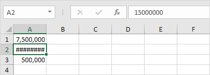
1. Click on the right border of the column A header and increase the column width.
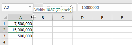
Tip: double click the right border of the column A header to automatically fit the widest entry in column A.
#NAME? error
The #NAME? error occurs when Excel does not recognize text in a formula.
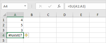
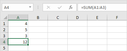
1. Simply correct SU to SUM.
#VALUE! error
Excel displays the #VALUE! error when a formula has the wrong type of argument.
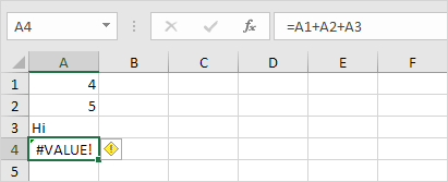
1a. Change the value of cell A3 to a number.
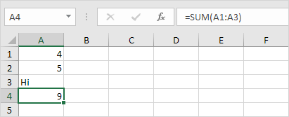
1b. Use a function to ignore cells that contain text.
#DIV/0! error
Excel displays the #DIV/0! error when a formula tries to divide a number by 0 or an empty cell.
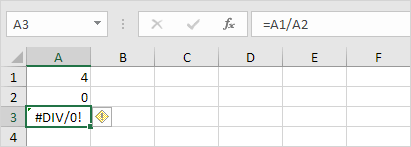
1a. Change the value of cell A2 to a value that is not equal to 0.
1b. Prevent the error from being displayed by using the logical function IF.
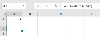
Explanation: if cell A2 equals 0, an empty string (“”) is displayed. If not, the result of the formula A1/A2 is displayed.
#REF! error
Excel displays the #REF! error when a formula refers to a cell that is not valid.
1. Cell C1 references cell A1 and cell B1.

2. Delete column B. To achieve this, right click the column B header and click Delete.
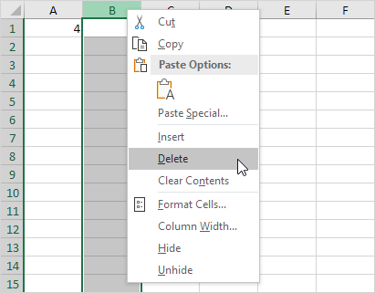
3. Select cell B1. The reference to cell B1 is not valid anymore.

4. To fix this error, you can either delete +#REF! in the formula of cell B1 or you can undo your action by pressing CTRL + z
IfError
This example illustrates the IFERROR function in Excel.
1. For example, Excel displays the #DIV/0! error when a formula tries to divide a number by 0.

2. Use the IFERROR function. If a cell contains an error, an empty string (“”) is displayed.

IsError
This example illustrates the ISERROR function in Excel.
1. For example, Excel displays the #DIV/0! error when a formula tries to divide a number by 0.
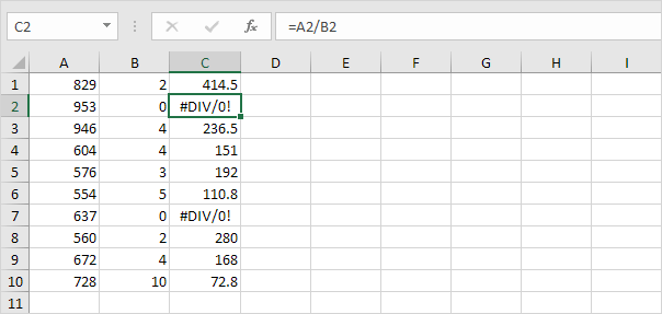
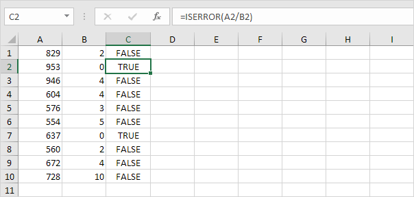
The ISERROR function checks whether a value is an error and returns TRUE or FALSE.
2. Use the IF and the ISERROR function. If a cell contains an error, the value 5 is returned. If not, the value 100 is returned.
Aggregate
Excel functions such as SUM, COUNT, LARGE and MAX don’t work if a range includes errors. However, you can easily use the AGGREGATE function to fix this.
1. For example, Excel returns an error if you use the SUM function to sum a range with errors.
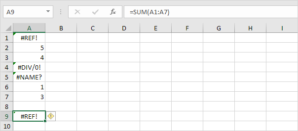
2. Use the AGGREGATE function to sum a range with errors.
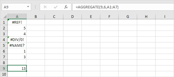
Explanation: the first argument (9) tells Excel that you want to use the SUM function. The second argument (6) tells Excel that you want to ignore error values.
3. It’s not easy to remember which argument belongs to which function. Fortunately, the AutoComplete feature in Excel helps you with this.
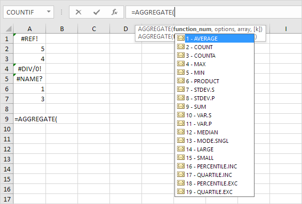
4. The AGGREGATE function below finds the second largest number in a range with errors.
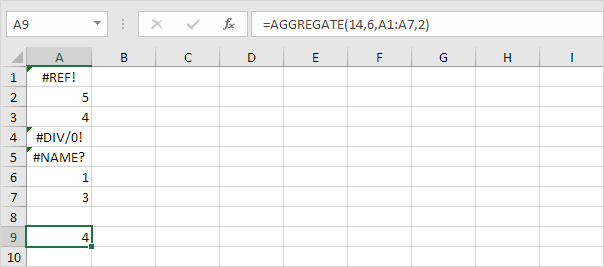
Explanation: the first argument (14) tells Excel that you want to use the LARGE function. The second argument (6) tells Excel that you want to ignore error values. The fourth argument (2) tells Excel that you want to find the second largest number.
5. The AGGREGATE function below finds the maximum value ignoring error values and hidden rows.
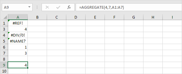
Explanation: the first argument (4) tells Excel that you want to use the MAX function. The second argument (7) tells Excel that you want to ignore error values and hidden rows. In this example, row 2 is hidden.
Circular Reference
A formula in a cell that directly or indirectly refers to its own cell is called a circular reference. This is not possible.
1. For example, the formula in cell A3 below directly refers to its own cell. This is not possible.
Note: Excel returns a 0 if you accept this circular reference.
2a. For example, the formula in cell C2 below refers to cell C1.

2b. The formula in cell C3 refers to cell C2.

2c. The formula in cell C4 refers to cell C3.

2d. So far, everything’s OK. Now change the value in cell C1 to the formula =C4. Cell C1 refers to cell C4, cell C4 refers to cell C3, cell C3 refers to cell C2, and cell C2 refers to cell C1. In other words, the formula in cell C1 indirectly refers to its own cell. This is not possible.

Note: Excel returns a 0 if you accept this circular reference.
3. To find your circular references, on the Formulas tab, in the Formula Auditing group, click the down arrow next to Error Checking.

4. Click Circular References.

Floating Point Errors
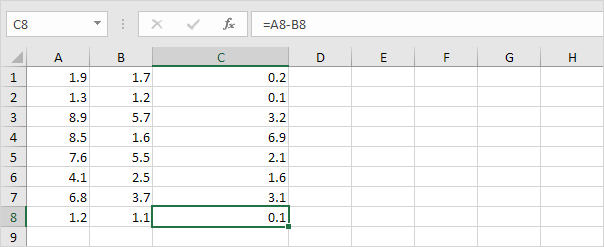
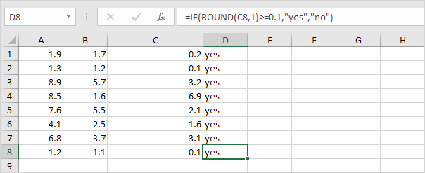
Excel stores and calculates floating point numbers. Sometimes, the result of a formula is a very close approximation.
1. For example, take a look at the formulas below. At first glance, everything looks alright.
Hope this helps! Leave a comment if this post helped you or in case of any questions.