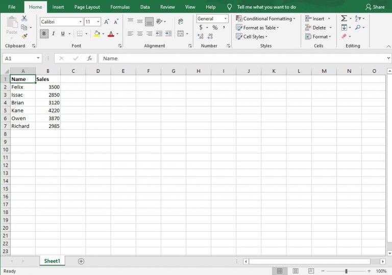
The data in Excel may need to be flipped sometimes i.e. to reverse the order of the data in a vertical dataset or a horizontal data set. Excel does not have an inbuilt feature to do this. Although there are multiple ways to do this using simple sorting tricks, formulas, or VBA. Here is the guide to flip data in excel using the SORT and helper column. This is one of the easiest ways to reverse the order of the dataset in excel.
Procedure To Flip Data Using SORT And Helper Column
Flip Data Vertically (Upside Down)
- Suppose there is a dataset of names in a column as shown below.

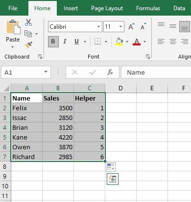
- Enter “Helper” as the heading for the column in the adjacent column.

- Enter a series of numbers (1,2,3,…) in the helper column.
 Select the entire dataset (including the helper column).
- Click on the data tab.

- Then click on the sort icon.
- Select “Helper” in the sort by option from the dropdown in the sort dialog box.

- Select “Largest to Smallest” in the Order dropdown.

- Then click OK.

- You can delete the helper’s column once done.
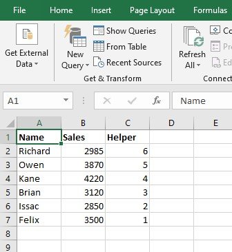
Here only the data of one column is flipped, but this technique can be used for an entire table. Make sure to select the entire table and then flip.
Flip Data Horizontally
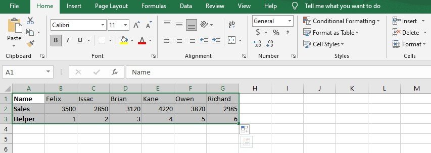
- Make a row with the heading “helper”.

- Then add a series of numbers in the row (1,2,3,…).
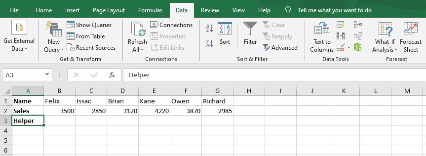
- Select the entire dataset (including the helper row).
- Click on the data tab.
- Then click on the sort icon.

- Click on the option buttons in the dialog box.
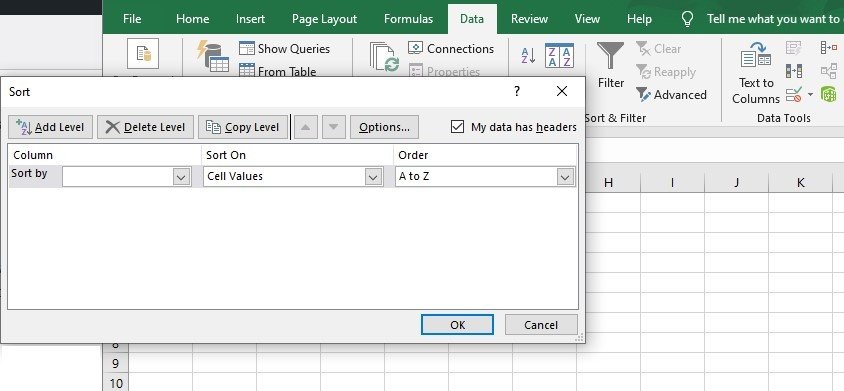
- Select orientation as “Sort left to right”.

- Then click OK.

- Select Row 3 (Hepler column row) in the sort dropdown.
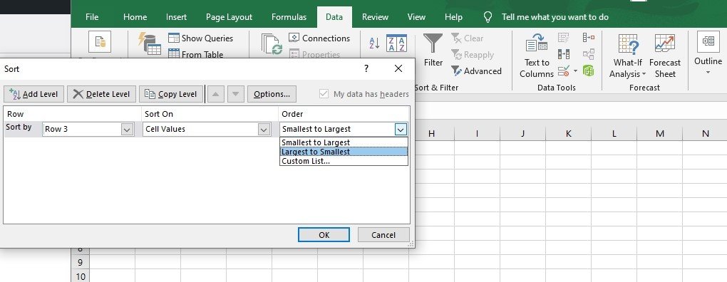
- Then select “Largest to Smallest” in the Order drop-down.

- Then click OK.