Lookup & Reference functions help you to work with arrays of data, and are particularly useful when you need to cross reference between different data sets. They perform tasks such as providing information about a range, returning the location of a given address or value, or looking up specific
Lookup & Reference (Index & Match) Functions
Vlookup
The VLOOKUP (Vertical lookup) function looks for a value in the leftmost column of a table, and then returns a value in the same row from another column you specify.
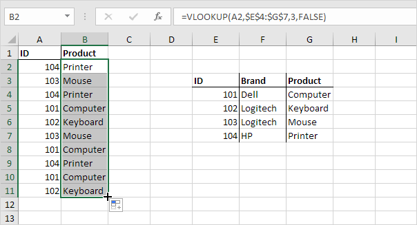
1. Insert the VLOOKUP function shown below.

Explanation: the VLOOKUP function looks for the ID (104) in the leftmost column of the range $E$4:$G$7 and returns the value in the same row from the third column (third argument is set to 3). The fourth argument is set to FALSE to return an exact match or a #N/A error if not found.
2. Drag the VLOOKUP function in cell B2 down to cell B11.

Note: when we drag the VLOOKUP function down, the absolute reference ($E$4:$G$7) stays the same, while the relative reference (A2) changes to A3, A4, A5, etc.
Hlookup
In a similar way, you can use the HLOOKUP (Horizontal lookup) function.

Match
The MATCH function returns the position of a value in a given range.

Explanation: Yellow found at position 3 in the range E4:E7. The third argument is optional. Set this argument to 0 to return the position of the value that is exactly equal to lookup_value (A2) or a #N/A error if not found.
Index
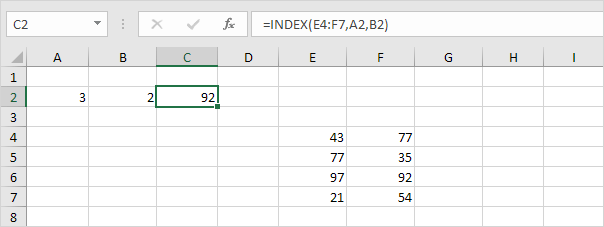
The INDEX function below returns a specific value in a two-dimensional range.

Explanation: 92 found at the intersection of row 3 and column 2 in the range E4:F7.
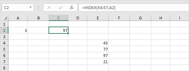
The INDEX function below returns a specific value in a one-dimensional range.

Explanation: 97 found at position 3 in the range E4:E7.
Choose
The CHOOSE function returns a value from a list of values, based on a position number.

Explanation: Boat found at position 3.
Hope this helps! Leave a comment if this post helped you or in case of any questions.